Simulation of realistic powder X-ray diffraction patterns
This post shows how to utilize the python-powder-diffraction package to simulate realistic powder XRD patterns.
Powder XRD patterns
X-ray diffraction (XRD) is a popular method to analyze crystalline sampes. In practice, the sample is often ground into a fine powder to analyze the sample from all directions simultaneously without the need to rotate the sample. Thus, the data is recorded as pairs of angles (typically \(2θ\)) and corresponding intensities. These diffraction patterns provide valuable information about the crystal structure, including lattice spacing and symmetry. Furthermore, the pattern contains information regarding the specimen, such as the size of grains in the powder.
Depending on the chemical composition and arrangement within the resulting crystal structure, each material exhibits a unique diffraction pattern characterized by specific peak intensities and positions. As a result, the diffraction pattern serves as a distinctive fingerprint that can be used to identify materials present in the recorded data. By comparing experimental diffraction patterns with known reference patterns stored in databases, scientists can accurately determine the composition and structure of the crystalline sample under investigation. Therefore, XRD is widely employed in various domains to rapidly identify known materials and ensure quality control, while also playing a crucial role in research to determine the properties of novel materials.
Appearance
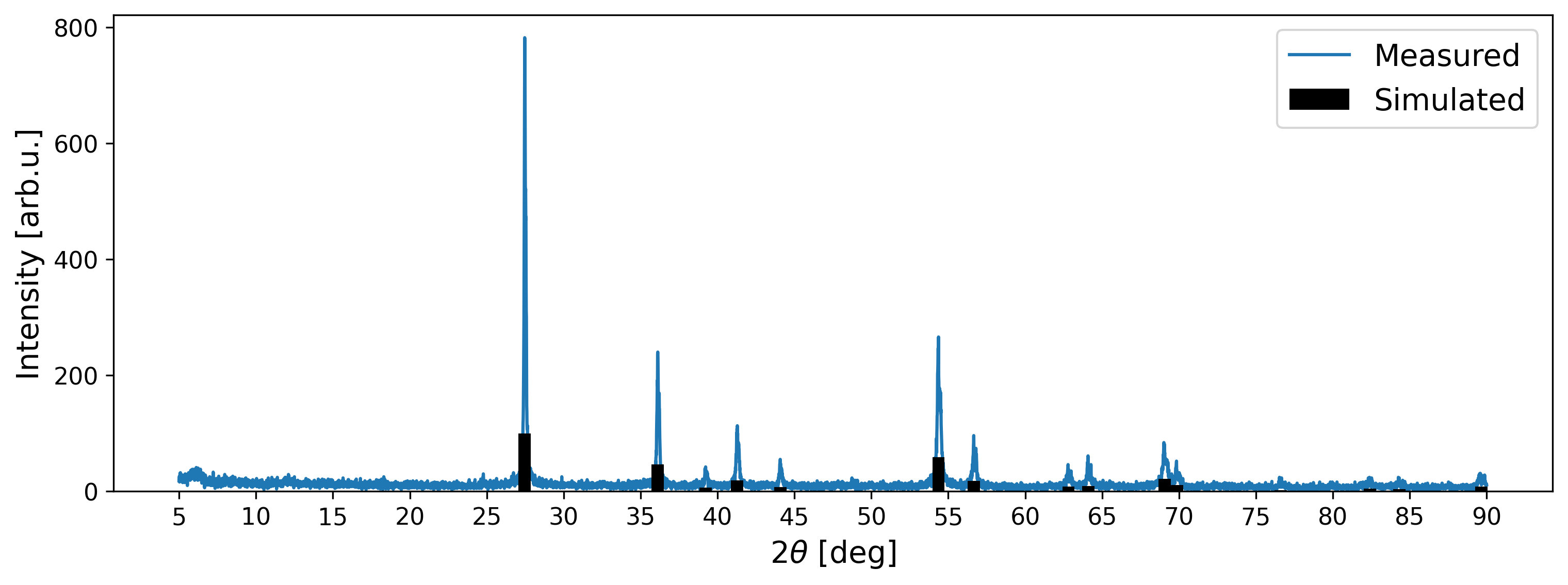
The following figure shows an exemplary XRD pattern that has been acquired from the RRUFF database. In particular, entry R050031 has been selected, which corresponds to the mineral rutile. This substance with chemical composition TiO2 and a tetragonal crystal structure has been analyzed using a XRD instrument with a copper anode (wavelength 0.1540562 nm), resulting in the following pattern:
The signal displays multiple peaks (e.g., at positions 27, 36, and 54 degrees \(2θ\)), each exhibiting a broad shape. Additionally, the signal exhibits noise and artifacts, such as the bump observed at the beginning of the measurement, which do not correspond to the characteristic diffraction pattern of the rutile sample. These discrepancies may be attributed to various factors collectively referred to as “background”. The analysis of the acquired diffraction pattern enabled the determination of lattice parameters, as reported: \(a = b = 4.5945; c = 2.9594\).
Reported Information
While the RRUFF database offers measured XRD patterns for certain minerals, the data extracted from these diffraction patterns is generally stored in a condensed format. Databases like the COD or the ICSD have thousands of entries, containing comprehensive information on chemical composition and crystal structure arrangement. These databases also offer the option to download the structural information, often in the form of crystallographic information files (CIFs), which allows researchers to utilize the data for subsequent analysis and simulations.
Pattern Simulation
Utilizing the condensed information, calculating the corresponding positions and intensities of diffraction peaks for a given structure becomes a straightforward process. Therefore, this method has been incorporated into numerous software packages, including those designed for the Search/Match procedure and various scientific applications. For the purposes of this post, the implementation provided by pymatgen is utilized, though alternative options such as cctbx are also available. An overview of commercial and free-to-use Search/Match software is given here.
Requirements
In order to utilize the Python package pymatgen, several prerequisites are required:
- A fresh Python environment, e.g., through venv or conda.
- The installation of pymatgen and required packages through
pip install pymatgen. - A CIF of the structure to simulate, here a rutile structure from the COD 9015662.
Procedure
First, read the CIF. The pymatgen modules interpret this information and represent it as follows:
from pymatgen.core import Structure
struct = Structure.from_file('Downloads/9015662.cif')
print(struct)
Structure Summary
Lattice
    abc : 4.5937 4.5937 2.9587
 angles : 90.0 90.0 90.0
 volume : 62.434723178803
      A : 4.5937 0.0 2.8128300006215983e-16
      B : 7.387233015819564e-16 4.5937 2.8128300006215983e-16
      C : 0.0 0.0 2.9587
    pbc : True True True
PeriodicSite: Ti (0.0000, 0.0000, 0.0000) [0.0000, 0.0000, 0.0000]
PeriodicSite: Ti (2.2969, 2.2969, 1.4794) [0.5000, 0.5000, 0.5000]
PeriodicSite: O (1.4001, 1.4001, 0.0000) [0.3048, 0.3048, 0.0000]
PeriodicSite: O (3.1936, 3.1936, 0.0000) [0.6952, 0.6952, 0.0000]
PeriodicSite: O (3.6969, 0.8968, 1.4794) [0.8048, 0.1952, 0.5000]
PeriodicSite: O (0.8968, 3.6969, 1.4794) [0.1952, 0.8048, 0.5000]
This demonstrates that the dimensions and arrangement of the crystal structure have been processed, as the Structure instance does not include every single Ti and O site in the unit cell. Instead, the remaining positions are represented using the PeriodicSite object. Furthermore, this shows that the lattice dimensions of the rutile structure from the COD differ slightly from the RRUFF entry.
To calculate the diffraction pattern information, pymatgen provides the XRDCalculator module, which computes the positions and intensities (scaled according to the highest peak) for a given structure as follows:
from pymatgen.analysis.diffraction.xrd import XRDCalculator
calc = XRDCalculator(wavelength="CuKa")
pattern = calc.get_pattern(struct, two_theta_range=(5., 90.))
The pattern object contains the discrete peak positions (pattern.x) and peak intensities (pattern.y).

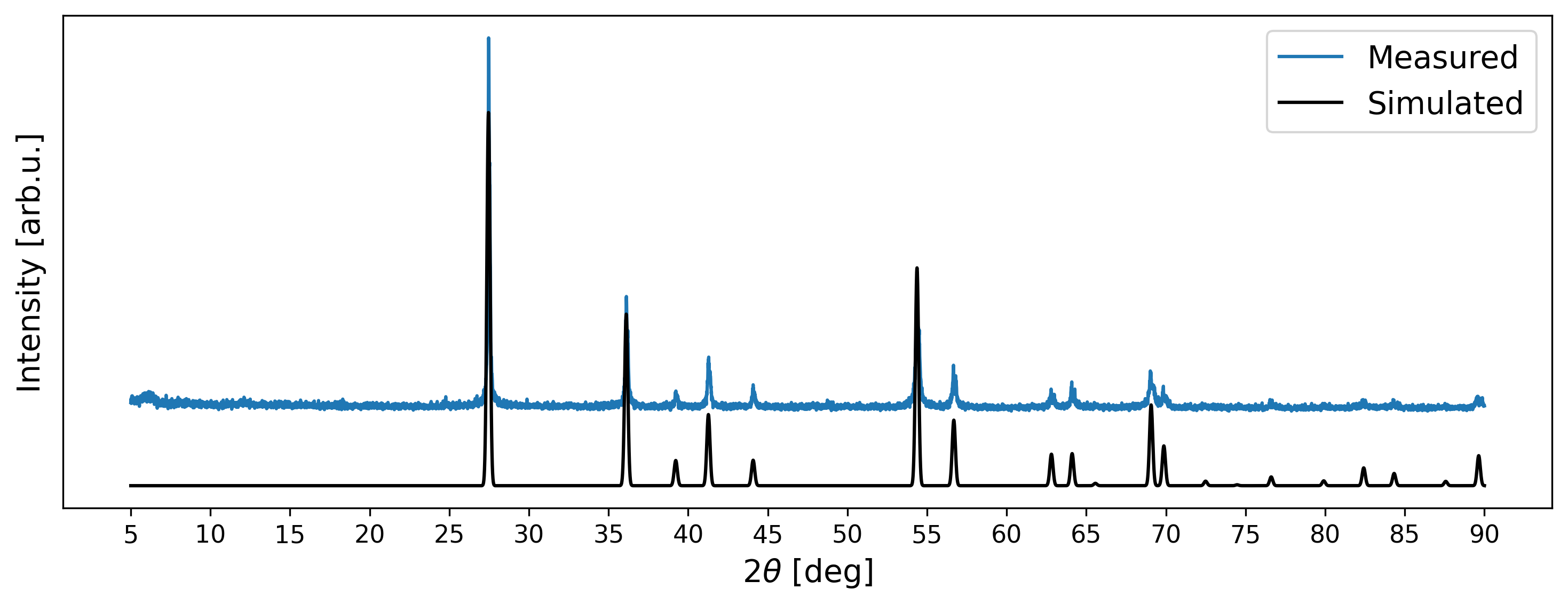
A visual comparison between the simulated data and the measured XRD pattern validates that the peak positions align. However, notable disparities arise in the intensities: while the highest peak in the measured signal registers at approximately 800 arb. u., the simulated peaks are scaled relative to the highest peak at 100 arb. u. The measured intensities are influenced by various factors, such as instrument configuration and acquisition time. As a result, XRD patterns are commonly analyzed based on the relative intensities captured in the signal. A straightforward method to align the scales of measured and simulated intensities involves scaling based on the minimum and maximum values in each scan, known as Min-Max-Scaling.
Furthermore, while the measured peaks exhibit broad shapes, the XRDCalculator module computes only discrete positions. Consequently, additional steps are necessary to modify the calculated diffraction peaks to match the broadened nature of the measured signal. This can be achieved by convolving the peaks with a kernel that approximates a probability distribution (centered at 0). In practice, peak shapes commonly display a Voigt profile. Alternatively, convolution with a Gaussian profile is also feasible and computationally less demanding.
Prior to the convolution, it is essential to map the discrete peak positions onto a signal with a defined scanning range and equidistant measurement steps. The measured XRD pattern was obtained within a scanning range spanning from 5 to 90 degrees \(2θ\), with a step width of 0.01 degrees \(\Delta2θ\). Therefore, the calculated peaks are aligned with these measurement steps accordingly.
import numpy as np # represent the simulated signal as a numpy vector

# measurement steps
steps = np.linspace(5., 90., 8501, endpoint=True)
# initiliaze signal with all values equal to zero
signal = np.zeros_like(steps)

angles, intensities = pattern.x, pattern.y

# iterate over the computed angles
for i, ang in enumerate(angles):
    # determine index of measured step for mapping
    idx = np.argmin(np.abs(ang - steps))
    # place peak with corresponding intensity in signal
    signal[idx] = intensities[i]

from scipy.ndimage import gaussian_filter1d

signal = gaussian_filter1d(signal, 10., mode="constant")

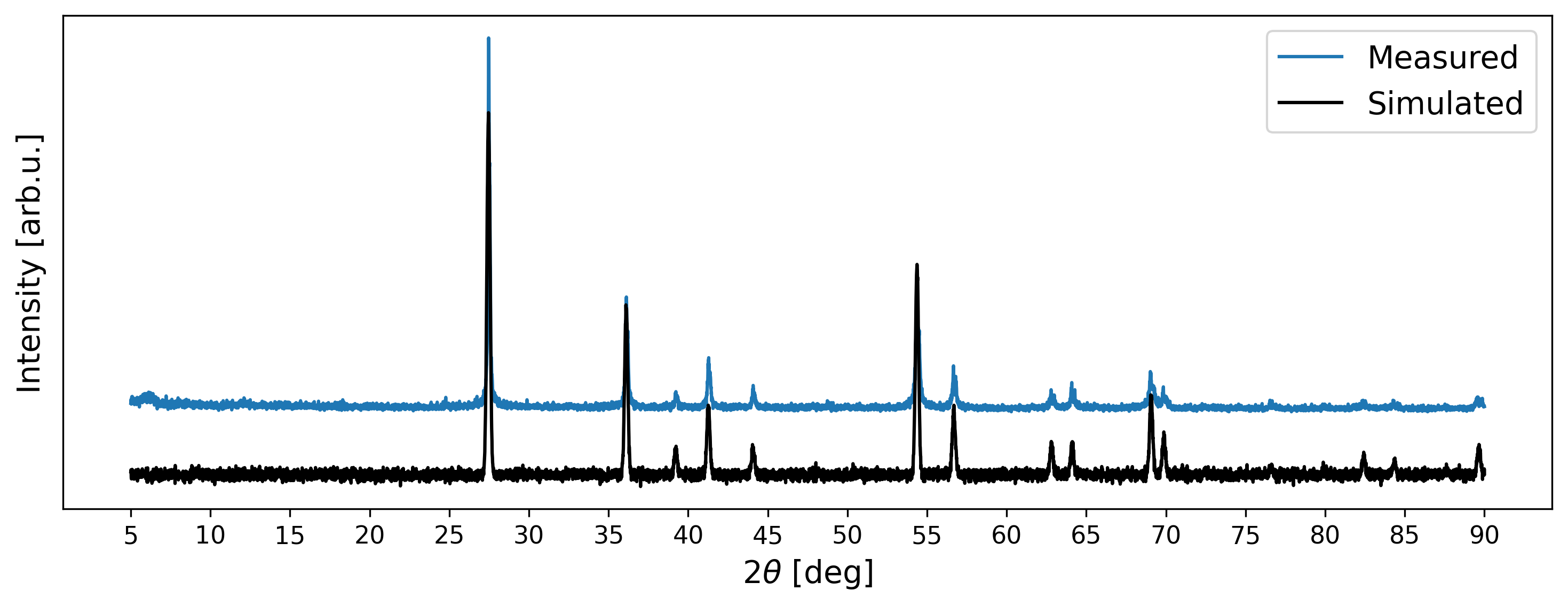
What is missing now? Mostly the noise and background intensities found in measured signals. In most Search/Match applications, background is modeled through Chebyshev polynomials and noise can be added through random sampling of values from a normal distribution (white noise). Both procedures are straightforward to accomplish in Python:
coefs = [0., 0., 0., 0.] # coefficients for Chebyshev polynomial
chebyshev = np.polynomial.chebyshev.Chebyshev(ccoefs)
# evaluate the polynomial according to the measurement steps
background = chebyshev.linspace(steps.size)[1]

# set seed for reproducability
rng = np.random.default_rng(2024)
noise = rng.normal(0, 0.033, steps.size)

# add to signal, background not needed here
signal += noise

Python-Powder-Diffraction
Exemplary Use
Instead of manually implementing the code described above, an artificial diffraction pattern can also be generated using the python-powder-diffraction package:
from powdiffrac import Powder
from powdiffrac.simulation import generate_noise
powder = Powder.from_cif('Downloads/9015662.cif')
signal = powder.get_signal()
signal = generate_noise(signal)
Pattern Variation
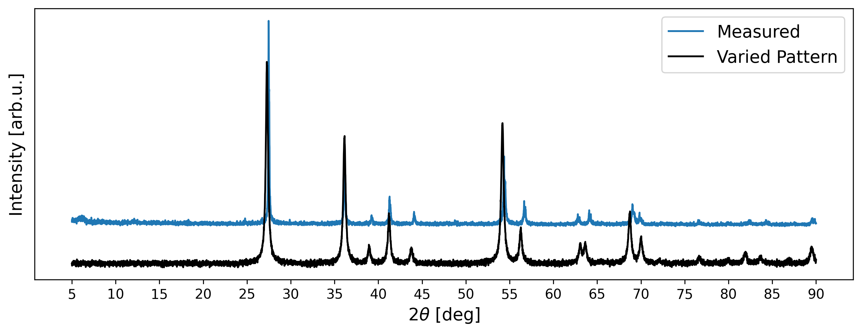
Although the generated XRD pattern looks visually similar to the measured signal, minor disparities persist. Firstly, there are slight deviations in peak positions attributable to a mismatch in lattice parameters. Secondly, certain simulated intensity peaks exceed the intensities observed in the measured data. Thirdly, disparities are evident in the shapes of peaks. Nonetheless, such deviations have to be expected in measured diffraction patterns.
The Powder object furthermore includes functionality to generate varied signals. For example, the following code generates a pattern with varied peak positions, intensities, and shapes.
powder = Powder.from_cif(
    'Downloads/9015662.cif',
    two_theta = (5.,90.),
    max_strain = 0.04, # position variation
    max_texture = 0.6, # intensity variation
    min_domain_size = 10, # minimum grain size 10nm
    max_domain_size = 50, # maximum grain size 100nm
    peak_shape: str = "lorentzian", # desired peak shapes
    vary_strain = True,
    vary_texture = True,
    vary_domain = True,
    seed = 2024
)
signal = powder.get_signal(vary=True)
signal = generate_noise(signal)
