Training a neural network for the classification of TiO2 XRD patterns
This post demonstrates the usage of neural networks for automatic analysis of powder XRD data. In this application, the objective is to identify various TiO2 structures based on their characteristic pattern.
Titanium Oxides
Titanium oxide TiO2 can crystallize in various arrangements, depending on diverse influences. According to crystalline databases, such as the COD or the ICSD, there are 5 major phases to consider at ambient conditions:
- Anatase, e.g., COD 9009086
- Rutile, e.g., COD 9015662
- Brookite, e.g., COD 8104269
- β-TiO2, e.g., COD 1528778
- TiO2-II, e.g., COD 1530026
While the chemical composition for all of these phases is identical, their crystalline structures differ. Therefore, the XRD technique is a useful method to determine the exact phase for titanium oxide samples.

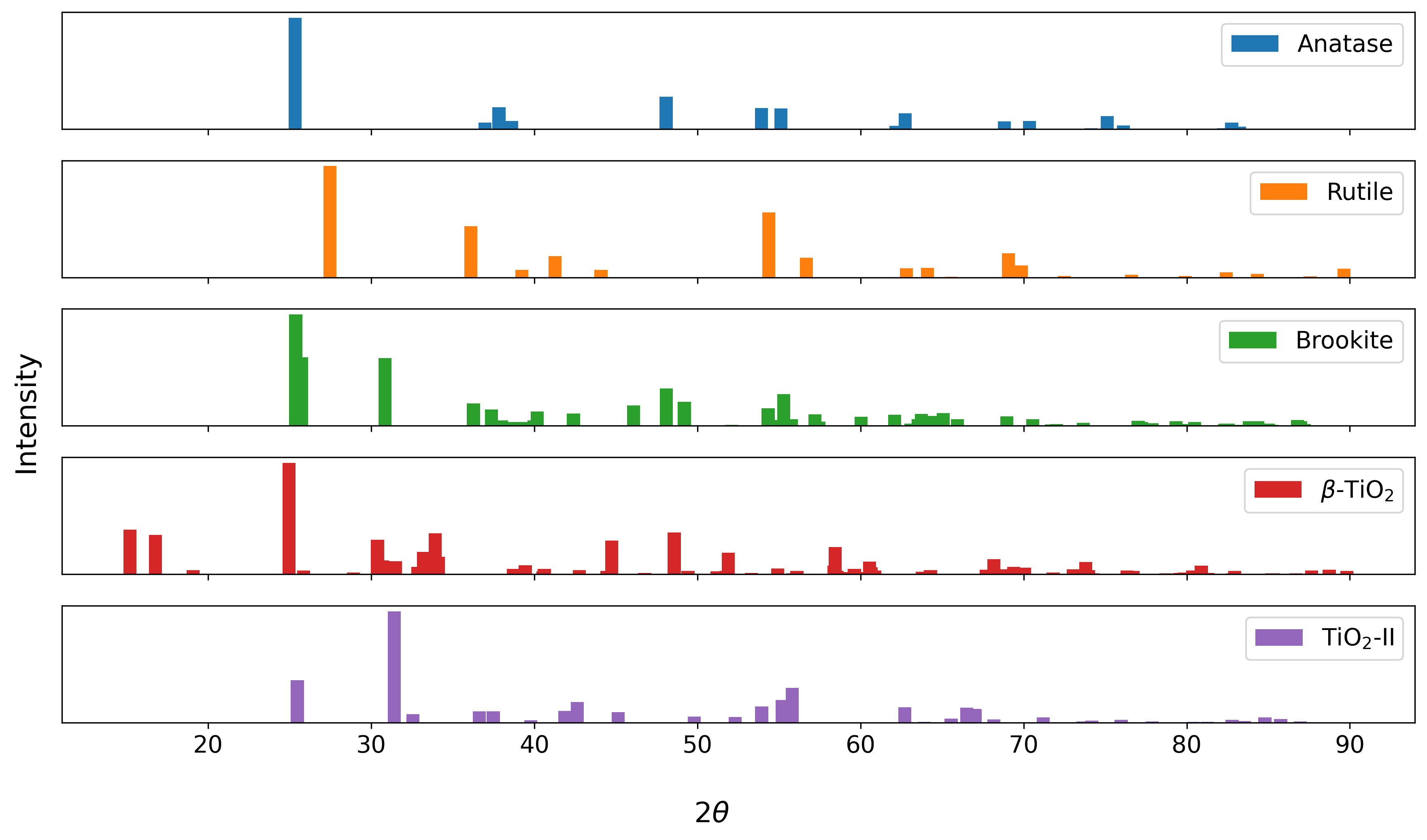
The above figure shows the simulated, ideal diffraction patterns for the different structures. While the highest peak lies in the range between 25 and 30 degrees \(2θ\) for 4 of the 5 variants (TiO2-II being the exception), the structures are distinguishable based on the presence and positions of additional diffraction peaks. Therefore, it can be expected that an automated classification algorithm is able to classify the structures accordingly.
Network Training
The use of neural networks for analysis of powder XRD patterns has been demonstrated in various publications.1,2 Nonetheless, exemplary data is necessary to train the network models. This data should demonstrate all types of variations found in the powder XRD patterns, so the model can learn robust classification rules for the different structures. However, measured XRD patterns are not readily available for all types of materials. Thus, simulated XRD patterns are typically utilized as training data. The previous blog post explains the procedure in detail using the python-powder-diffraction package.
Requirements
- A fresh Python environment, e.g., through venv or conda.
- CIFs for the different TiO2 variants, e.g., from the COD.
- The python-powder-diffraction package installed in the environment.
- A deep learning package, such as TensorFlow or PyTorch installed in the environment.
Data Generation
The python-powder-diffraction provides several methods to generate varied patterns for each structure, but the fastest option is the use of the generate-varied-patterns script provided in the package. Simply place all CIFs in a folder (e.g., in a directory called phases), activate the enviroment and use generate-varied-patterns phases to generate the signals.
Furthermore, there are several arguments to modify the data generation procedure. Here, we’re aiming to simulate patterns in the 5 to 90 degrees \(2θ\) range with step width \(0.01^\circ \Delta 2\theta\). To depict the peak positions, intensities, and shape variations, we also specify values for those parameters:
generate-varied-patterns phases --theta_range "(5,90)" --strain 0.04 --texture 0.8 --domain_sizes "(20,50)" --n_train 100 --n_val 20
Executing this script generates four numpy files in the phases directory: x_train.npy, x_val.npy, y_train.npy, and y_val.npy. The x arrays contain the signals (100 or 20 variants for each CIF) and the y arrays the labels for each pattern. By default, the CIFs are sorted according to their name and given an identifier in ascending order. Therefore, the labels file only contains the numerical identifier that specifies the structure for each signal in the train and val files.
Furthermore, the artificial signals should also contain background and noise. This can be added using the add-noise script. Noise can either be added to each signals array separately or in a single script execution using the --template argument. To add noise in a single call, we change the directory to the phases folder and call the script as follows:
add-noise --template "x_" --noise_min 0.01 --noise_max 0.05
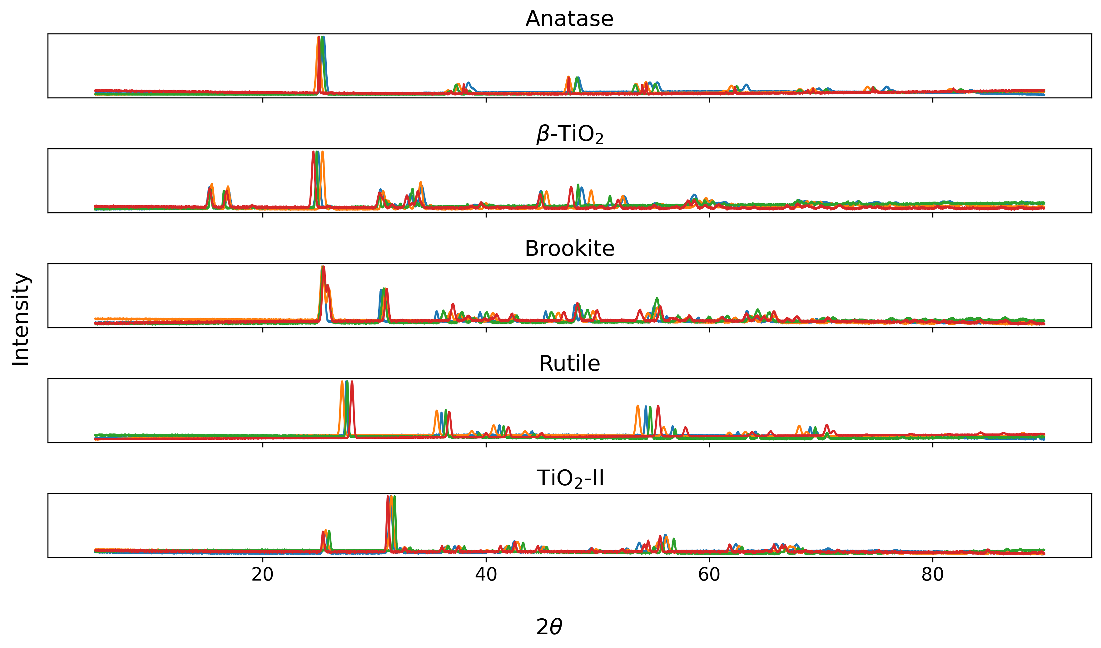
This call adds random background and noise to the x_train.npy and x_val.npy files and saves the modified arrays as x_train_noise.npy and x_val_noise.npy. The resulting signals appear as follows:

Neural Network
Convolutional neural networks employ various filters that are shifted across the input to identify features in the signals. Therefore, this architecture is well suited to distinguish the relevant peak-encoded information from background and noise. Here, we use a simple network consisting of three convolutional layers. Each generated signal corresponds to one of the unique structures, which represents a multi-class task. Therefore, the output of the network has five neurons and the outputs are scaled using the softmax activation function, to represent the predicted values as a probability distribution.
The neural network model, in this example using the keras implementation with a tensorflow backend, can be defined as follows:
from tensorflow.keras import Model, layers, metrics

def get_cnn(input_size=8501, classes=5):
    input_layer = layers.Input(shape=(input_size, 1),
                               name="input")
    x = layers.Conv1D(16, 35, padding='same',
                      activation='relu')(input_layer)
    x = layers.MaxPool1D()(x)
    x = layers.Conv1D(16, 25, padding='same',
                      activation='relu')(x)
    x = layers.MaxPool1D()(x)
    x = layers.Conv1D(16, 15, padding='same',
                      activation='relu')(x)
    x = layers.MaxPool1D()(x)
    x = layers.Flatten(name='flat')(x)
    x = layers.Dense(50, activation='relu')(x)
    out = layers.Dense(classes, activation='softmax')(x)
    model = Model(input_layer, out)
    model.compile(optimizer="adam", loss='sparse_categorical_crossentropy',
                  metrics=[metrics.SparseCategoricalAccuracy(name='accuracy')])
    return model
This implements a model with 8501 input neurons and 5 neurons in the output layer. Three convolutional layers with 16 filters each (and kernel sizes 35, 25, and 15) are employed within the network, together with pooling operations to reduce the dimensionality of the signals. The label files y_train.npy and y_val.npy specify the identifiers of each class, so the sparse_categorical_crossentropy loss (and accuracy object) is used. Furthermore, the Adam optimizer is used during model training.
Training Procedure
The next step involves the training of the neural network using the simulated patterns. Therefore, the first steps of the training script involve loading the signals.
import numpy as np
from tensorflow.keras import callbacks
from powdiffrac.processing import scale_min_max
from model import get_cnn


xt = scale_min_max(np.load("./phases/x_train.npy"))
xv = scale_min_max(np.load("./phases/x_val.npy"))
yt = np.load("./phases/y_train.npy")
yv = np.load("./phases/y_val.npy")
Following this, the model can get initiliazed based on the properties of the training data. Consisting of 5 unique classes, adapting the model to the training data requires only few epochs.
model = get_cnn(input_size=xv.shape[1], classes=np.unique(yv).size)
model.fit(xt, yt, batch_size=32, epochs=10, verbose=2, validation_data=(xv, yv), shuffle=True)
model.save("./phases/model.keras")
In my configuration (GTX 1070), the model achieves 100% accuracy on training and validation set. This is especially remarkable because the model has never seen the varied patterns in the validation data.
Epoch 10/10
16/16 - 0s - loss: 1.3780e-07 - accuracy: 1.0000 - val_loss: 4.3869e-07 - val_accuracy: 1.0000 - 209ms/epoch - 13ms/step
Network Application
While the model has been trained and evaluated on simulated patterns, it is also readily applicable for the classification of measured powder XRD patterns. Therefore, the following section demonstrates the performance of the neural network model on measured signals.
RRUFF Measurements
The RRUFF database provides measured XRD patterns and Raman spectra for various materials. This database includes entries for some of the TiO2 variants, enabling an effective evaluation of the trained neural network model using measured signals. The database includes the following entries:
| Phase | Entries | … | … | … |
|---|---|---|---|---|
| Anatase | R060277 | R070582 | R120013 | R120064 |
| Rutile | R040049 | R050031 | R050417 | R060493 |
| Brookite | R050363 | R050591 | R130225 |
Unfortunately, the entries for the four Anatase samples do not contain measured XRD patterns and the database only provides simulated signals. Nonetheless, the process to generate those simulated patterns presumably differs from the approach to generate the training signals, so this is another useful tool to test the robustness of the automated analysis approach.
Prediction
The measured patterns are available for download from the RRUFF, enabling the evaluation of the trained model in a Python script. Accordingly, the scans are imported into Python (using numpy functions) and Min-Max-scaled prior to feeding the signals into the network. The order of the signals corresponds to the table above, meaning that signals 1-4 represent anatase, signals 5-8 represent rutile, and the remaining depict brookite.
model = tf.keras.models.load_model("./phases/model.keras")
anatase_1 = np.loadtxt('./meas/Anatase__R060277-9__Powder__Xray_Data_XY_RAW__5487.txt', comments='#', delimiter=',')
...
meas = np.zeros([11,8501])
meas[0] = np.interp(np.linspace(5.,90.,8501), anatase_1[:,0], anatase_1[:,1])
...
meas = scale_min_max(meas)
prediction = model.predict(meas)
np.argmax(prediction, axis=1)
array([0, 0, 0, 0, 3, 3, 3, 3, 2, 2, 2])
The network provides the correct predictions for the measured signals (identifiers-> 1: Anatase, 2: β-TiO2, 2: Brookite, 3: Rutile, 4: TiO2-II), corresponding to an accuracy score of 100%.
Limitations
While the network demonstrates proficiency in classifying XRD patterns of titanium oxide samples, there are several other cases that can occur when analyzing a crystalline sample. For once, the sample could contain several phases, such as impurities. Secondly, the sample could contain neither of the defined phases. The network presented here is not trained to handle either of these exceptional cases. Accordingly, the network classified the first rutile sample from the RRUFF (R040049) as rutile, despite the presence of hematite in the sample (as indicated in the RRUFF entry). Due to the use of the softmax activation function in the final layer, the output with the highest value is typically interpreted as the predicted class, so the network does not have the option to reject a sample that fits neither of the five TiO2 phases.
References
-
Wang, H., et al. “Rapid identification of X-ray diffraction patterns based on very limited data by interpretable convolutional neural networks.” Journal of chemical information and modeling 60.4 (2020): 2004-2011. ↩
-
Schuetzke, J., et al. “Enhancing deep-learning training for phase identification in powder X-ray diffractograms.” IUCrJ 8.3 (2021): 408-420. ↩